This blogpost is about RStudio and the reticulate package! Reticulate includes a Python engine for R Markdown that enables easy interoperability between Python and R chunks. This enables us to bring the power of Earth Engine to RStudio.

Tutorial: Deriving simple tree phenology data from Sentinel2 with Earth Engine and plotting the data in R.

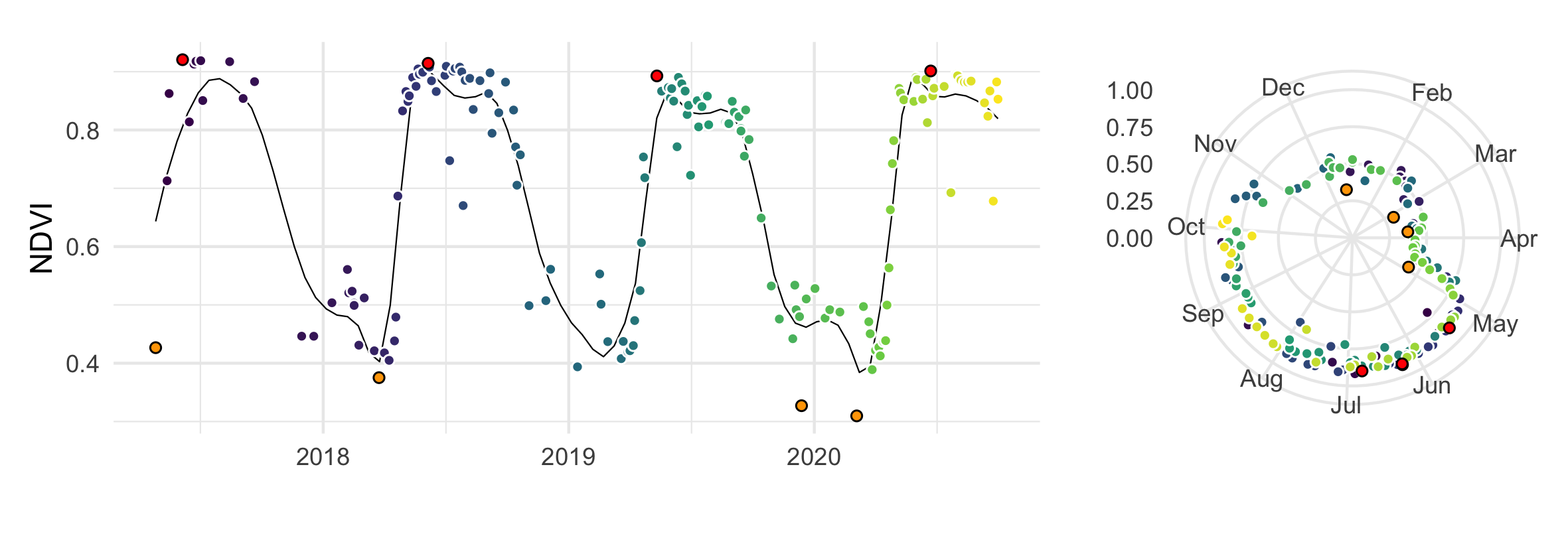Sentinel-2 derived NDVI values of a beech forest plotted over four years with annual min/max values highlighted.

Life between Use GoogleEarthEngine and in RStudio

Life between #GoogleEarthEngine and #R pic.twitter.com/ZbI33X21i3
— Hammad Gilani (@gilanius) October 14, 2020

With reticulate we can use:

the Google Earth Engine Python API to extract values of satellite data (in Python chunks),
dplyr & ggplot packages to manipulate the extracted data and to create e.g. a phenology chart (in R chunks).

My Setup

Mac - macOS High Sierra 10.13.6
R - version 3.6.3
RStudio - version 1.3.1093
Conda - version 4.7.12

Create new conda environment with earthengine-api

The RStudio Terminal provides access to the system shell from within the RStudio IDE. Open your Terminal tab and write:

### Terminal

# Create a conda environment
conda create --name gee-demo 

# Activate the environment
conda activate gee-demo      

# Install the Earth Engine Python API
conda install -c conda-forge earthengine-api 

# Authenticate your access with the command line tool
earthengine authenticate     

conda install pandas
conda install numpy

Create new R Markdown file

In RStudio, create a new R Markdown file (File => New File => R Markdown …) and install the reticulate package and apply the use_condaenv() function to point to the created ‘gee-demo’ conda environment.

### R

if(!require("reticulate")) install.packages("reticulate")
library(reticulate)

use_condaenv("gee-demo", conda = "auto",required = TRUE)

The Earth Engine Python API is available as a Python package that can be installed locally. The Python API package is called ee. It must be imported and initialized for each new Python session and script.

### Python

import ee       
ee.Initialize() # Initialize the API
print(ee.__version__)


## 0.1.238

At this point we have set up our working environment and can get started. The ultimate goal is to use this working environment and to visualize the phenology of a beech forest without leaving RStudio.

Generate NDVI data for a german beech forest

opentrees.org at 38.713521/-9.171883

With the help of the opentrees.org project I found a beech forest near Potsdam in East Germany. Opentrees.org is the world’s largest database of municipal street and park trees, produced by harvesting open data from dozens of different sources.

### Python

geometry = ee.Geometry.Polygon( # beech forest area
        [[[13.109782839513642, 52.42163736335469],
          [13.109782839513642, 52.420752422262055],
          [13.111671114660126, 52.420752422262055],
          [13.111671114660126, 52.42163736335469]]]);

Create a function to mask clouds using the Sentinel-2 QA band

### Python

def maskclouds(image):
    qa = image.select("QA60")
    cloudBitMask  = 1 << 10
    cirrusBitMask = 1 << 11
    mask  = qa.bitwiseAnd(cloudBitMask).eq(0) \
              .And(qa.bitwiseAnd(cirrusBitMask).eq(0))
    return image.updateMask(mask).divide(10000) \
                 .set('date', image.date().format()) # adding recording date

Create a function to add Normalized Difference Vegetation Index (NDVI) band

### Python

def ndvi(image):
    ndvi = image.normalizedDifference(["B8","B4"]).rename("ndvi")
    return image.addBands([ndvi])

Create two `ImageCollections` with Sentinel2 Level-2A and cloud probability data

### Python

start_date = ee.Date('2017-04-01')
end_date   = ee.Date('2020-12-31')

s2Sr = ee.ImageCollection("COPERNICUS/S2_SR") \
         .filterBounds(geometry) \
         .filterDate(start_date, end_date) \
         .filter(ee.Filter.eq('MGRS_TILE', '33UUU')) \
         .map(maskclouds) \
         .map(ndvi)

s2c = ee.ImageCollection('COPERNICUS/S2_CLOUD_PROBABILITY') \
        .filterBounds(geometry) \
        .filterDate(start_date, end_date);

Create a function to `Join` two collections on their ‘system:index’ property.

### Python

# The propertyName parameter is the name of the property
# that references the joined image.
def indexJoin(collectionA, collectionB, propertyName):
  joined = ee.ImageCollection(ee.Join.saveFirst(propertyName).apply(
    primary = collectionA,
    secondary = collectionB,
    condition = ee.Filter.equals(
      leftField = 'system:index',
      rightField = 'system:index'
    )
  ))
  # Merge the bands of the joined image.
  return joined.map(lambda image: image.addBands(ee.Image(image.get(propertyName)).rename("cld")))

Create a function to get a) median value and b) the recording date for each image

### Python

def calculateMedian(image):
  
  median = image.reduceRegion(reducer  = ee.Reducer.median(),
                            geometry = geometry,
                            scale = 10,
                            maxPixels = 1e9)

  # set the recording date and median values as a property of the image
  return image.set('date', image.get('date')).set('median', median)

Apply the `Join` function and median values

### Python

withCloudProbability = indexJoin(s2Sr, s2c, 'cloud_probability');

# select only the 'ndvi' and 'cloud probability' values. 
withMedian = withCloudProbability.select(["ndvi","cld"]).map(calculateMedian)

# reduce the images properties to a list of lists
values = withMedian.reduceColumns(ee.Reducer.toList(2), ['date', 'median']).values().get(0)

# Type casts the result into a List
eeList = ee.List(values)

# convert  list of lists to a dictionaty
medians = ee.Dictionary(eeList.flatten())

Call `getInfo()` on Earth Engine objects to get the object from the server to the client

### Python

median_values = medians.getInfo(); # ee.Dictionary => Python dictionary
type(median_values)

## <class 'dict'>

Python dictionary to pandas DataFrame

### Python

import pandas
pd_df = pandas.DataFrame.from_dict(median_values, orient='index')

STOP - lets see what we have got - STOP

### Python

pd_df

##                        cld      ndvi
## 2017-04-24T10:11:20   84.0       NaN
## 2017-04-27T10:20:25    9.0  0.426655
## 2017-05-04T10:13:49  100.0       NaN
## 2017-05-14T10:11:25   16.0  0.712856
## 2017-05-17T10:23:52    1.0  0.862517
## ...                    ...       ...
## 2020-09-30T10:16:16    6.0  0.852820
## 2020-10-03T10:26:13   67.0       NaN
## 2020-10-08T10:26:16   98.0       NaN
## 2020-10-10T10:16:16   99.0       NaN
## 2020-10-13T10:26:14  100.0       NaN
## 
## [457 rows x 2 columns]

In total we have NDVI and cloud probability data (from cloud free [0 %] to cloudy [100 %]) of 457 Sentinel-2 images in our DataFrame. Some rows have NaN values in the NDVI column. NaN values occur if clouds were recognized in the QA60 band and masked out.

Calling Python from R

The pd_df panda DataFrame, created within the Python chunk above, is available to R using the py object from the reticulate package.

### R

df <- py$pd_df # convert pandas DataFrame to R DataFrame
head(df)

##                     cld      ndvi
## 2017-04-24T10:11:20  84       NaN
## 2017-04-27T10:20:25   9 0.4266549
## 2017-05-04T10:13:49 100       NaN
## 2017-05-14T10:11:25  16 0.7128555
## 2017-05-17T10:23:52   1 0.8625174
## 2017-05-24T10:13:53 100       NaN

Prepare data for plotting

For the work with R we use the following packages:

### R

list.of.packages <- c("stringr", "dplyr", "tidyr", "ggplot2", "patchwork")
new.packages <- list.of.packages[!(list.of.packages %in% installed.packages()[, "Package"])]
if (length(new.packages)) install.packages(new.packages)

library(stringr)
library(dplyr)
library(tidyr)
library(ggplot2)
library(patchwork)

In the next code chunk we manipulate the data to make our life easier with the plotting. We extract the recording date from the rownames and additionally create year and doy (day of the year) values. We also delete all lines with NaN NDVI values and exclude images with cloud probability values greater than 40.

### R

xx <- df %>%
  mutate(row_names = rownames(df)) %>%
  mutate(datetime = stringr::str_split(row_names, "T", simplify = TRUE)[,1]) %>%
  select(-row_names) %>%
  drop_na(ndvi) %>%
  mutate(date = as.Date(datetime, format="%Y-%m-%d")) %>%
  filter(cld < 40) %>%
  mutate(yday = lubridate::yday(date)) %>%
  mutate(year = lubridate::year(date)) %>%
  mutate(id = 1:n())
  
str(xx)

## 'data.frame':	164 obs. of  7 variables:
##  $ cld     : num  9 16 1 2 21 22 11 7 16 4 ...
##  $ ndvi    : num  0.427 0.713 0.863 0.921 0.814 ...
##  $ datetime: chr  "2017-04-27" "2017-05-14" "2017-05-17" "2017-06-06" ...
##  $ date    : Date, format: "2017-04-27" "2017-05-14" ...
##  $ yday    : num  117 134 137 157 167 174 177 184 187 227 ...
##  $ year    : num  2017 2017 2017 2017 2017 ...
##  $ id      : int  1 2 3 4 5 6 7 8 9 10 ...



dim(xx)

## [1] 164   7

After filtering all NaN values and exclude cloud probabilities higher than 40 % we have 164 rows (median NDVI values) left to work with.

Plotting the data

### R

max <- xx %>%
  group_by(year) %>%
  filter(ndvi == max(ndvi)) 

min <- xx %>%
  group_by(year) %>%
  filter(ndvi == min(ndvi)) 

plot_title <- expression(paste("Phenology of a beech forest ", italic("(Fagus Sylvatica)"), " near Potsdam - Germany"))

plt1 <- ggplot(data = xx, aes(x = date, y = ndvi, fill = id)) + 
  geom_smooth(colour = "black", size=  0.25,se = FALSE, span = 0.15)+
  geom_point(colour = "white",pch=21) + 
  geom_point(data = max, aes(x = date, y = ndvi),fill = "red", pch = 21) +
  geom_point(data = min, aes(x = date, y = ndvi),fill = "orange", pch = 21) +
  ggtitle(plot_title) +
  xlab("") + ylab("Normalized Vegetation Index (NDVI)") +
  scale_fill_viridis_c() + theme_minimal() + theme(legend.position = "none") 

plt1

### R

plt2 <- ggplot(xx, aes(x=yday, y=ndvi, fill = id))+  
  coord_polar(theta="x", start=0,direction=1) +  
  geom_point(colour = "white", pch = 21) +  
  geom_point(data = max, aes(x = yday, y = ndvi),fill = "red", pch = 21) +
  geom_point(data = min, aes(x = yday, y = ndvi),fill = "orange", pch = 21) +
  scale_y_continuous(limits = c(0, 1)) +
  xlab("") + ylab("") +
  labs(caption = "Data - Sentinel2 | Processed - EarthEngine Python API") +
  scale_x_continuous(breaks = 30*0:11, minor_breaks = NULL, labels = month.abb) +
  scale_fill_viridis_c() + theme_minimal() + theme(legend.position = "none") 
 
plt2

### R

plt1 + plt2 + plot_layout(widths = c(2.5, 1), heights = unit(c(5), c('cm', 'null')))

Other examples

38.713521/-9.171883

Mediterranean cypress (Cupressus sempervirens) in Lisbon, Portugal

44.84549/-0.573493

Spanish plane (Platanus x hispanica) in Bordeaux, France

Session Info

### R

sessionInfo()

## R version 3.6.3 (2020-02-29)
## Platform: x86_64-apple-darwin15.6.0 (64-bit)
## Running under: macOS High Sierra 10.13.6
## 
## Matrix products: default
## BLAS:   /Library/Frameworks/R.framework/Versions/3.6/Resources/lib/libRblas.0.dylib
## LAPACK: /Library/Frameworks/R.framework/Versions/3.6/Resources/lib/libRlapack.dylib
## 
## locale:
## [1] en_US.UTF-8/en_US.UTF-8/en_US.UTF-8/C/en_US.UTF-8/en_US.UTF-8
## 
## attached base packages:
## [1] stats     graphics  grDevices utils     datasets  methods   base     
## 
## other attached packages:
## [1] patchwork_1.0.0 ggplot2_3.3.2   tidyr_1.1.0     dplyr_1.0.0    
## [5] stringr_1.4.0   reticulate_1.16
## 
## loaded via a namespace (and not attached):
##  [1] Rcpp_1.0.5        pillar_1.4.6      compiler_3.6.3    tools_3.6.3      
##  [5] digest_0.6.25     nlme_3.1-144      jsonlite_1.7.1    lubridate_1.7.9  
##  [9] evaluate_0.14     lifecycle_0.2.0   tibble_3.0.4      gtable_0.3.0     
## [13] lattice_0.20-38   viridisLite_0.3.0 mgcv_1.8-31       pkgconfig_2.0.3  
## [17] rlang_0.4.8       Matrix_1.2-18     yaml_2.2.1        xfun_0.18        
## [21] withr_2.3.0       knitr_1.30        generics_0.0.2    vctrs_0.3.4      
## [25] grid_3.6.3        tidyselect_1.1.0  glue_1.4.2        R6_2.4.1         
## [29] rmarkdown_2.3     farver_2.0.3      purrr_0.3.4       magrittr_1.5     
## [33] splines_3.6.3     scales_1.1.1      ellipsis_0.3.1    htmltools_0.5.0  
## [37] colorspace_1.4-1  labeling_0.3      stringi_1.5.3     munsell_0.5.0    
## [41] crayon_1.3.4

Bottom line

This blogpost showed you how to use Earth Engine Python API in RStudio. If you have any questions, suggestions or spotted a mistake, please use the comment function at the bottom of this page.

You can cite this blogpost using: Gärtner, Philipp (2020/10/16) “Use Google’s Earth Engine Python API in RStudio”, https://philippgaertner.github.io/2020/10/use-gee-python-api-in-rstudio/

Previous blog posts are available within the blog archive. Feel free to connect or follow me on Twitter - @Mixed_Pixels.

Use Google's Earth Engine Python API in RStudio

Life between Use GoogleEarthEngine and in RStudio

My Setup

Create new conda environment with earthengine-api

Create new R Markdown file

Generate NDVI data for a german beech forest

Create a function to mask clouds using the Sentinel-2 QA band

Create a function to add Normalized Difference Vegetation Index (NDVI) band

Create two `ImageCollections` with Sentinel2 Level-2A and cloud probability data

Create a function to `Join` two collections on their ‘system:index’ property.

Create a function to get a) median value and b) the recording date for each image

Apply the `Join` function and median values

Call `getInfo()` on Earth Engine objects to get the object from the server to the client

Python dictionary to pandas DataFrame

STOP - lets see what we have got - STOP

Calling Python from R

Prepare data for plotting

Plotting the data

Other examples

Session Info

Bottom line

Philipp Gärtner

Use Google's Earth Engine Python API in RStudio

Life between Use GoogleEarthEngine and in RStudio

My Setup

Create new conda environment with earthengine-api

Create new R Markdown file

Generate NDVI data for a german beech forest

Create a function to mask clouds using the Sentinel-2 QA band

Create a function to add Normalized Difference Vegetation Index (NDVI) band

Create two ImageCollections with Sentinel2 Level-2A and cloud probability data

Create a function to Join two collections on their ‘system:index’ property.

Create a function to get a) median value and b) the recording date for each image

Apply the Join function and median values

Call getInfo() on Earth Engine objects to get the object from the server to the client

Python dictionary to pandas DataFrame

STOP - lets see what we have got - STOP

Calling Python from R

Prepare data for plotting

Plotting the data

Other examples

Session Info

Bottom line

Philipp Gärtner

Create two `ImageCollections` with Sentinel2 Level-2A and cloud probability data

Create a function to `Join` two collections on their ‘system:index’ property.

Apply the `Join` function and median values

Call `getInfo()` on Earth Engine objects to get the object from the server to the client