
In Google Earth Engine we usually load an image collection first and then filter it by a date range, a region of interest and a image property with some cloud percentage estimates.
If the cloud threshold value is set too low it may happen that we throw away (filter out) to many images that could have been useful for our analysis. If we select the filter too generously, too many scenes with clouds remain. Finding a good threshold is not easy, this blog post may help to find it.
Sentinel2 - QA60 band
Each Sentinel-2 image has a bitmask band with cloud mask information - QA60. QA stands for quality while the 60 reveals the spatial resolution in meter. See the full explanation of how cloud masks are computed. Possible values are
- Bit 10: Opaque clouds
- 0: No opaque clouds
- 1: Opaque clouds present
- Bit 11: Cirrus clouds
- 0: No cirrus clouds
- 1: Cirrus clouds present
To get the respective bit values we use the Javascript bitwise left shift operator <<.
// Javascript

var cloudBitMask  = 1 << 10; // 1024
var cirrusBitMask = 1 << 11; // 2048
Now we only need one simple function to read the cloud, cirrus or cloud-free bit mask values from the QA60 band and add each cloud type as new band to our original image.
// Javascript

var addValues = function(image) {
  var cloud     = image.eq(cloudBitMask).rename('cloud');
  var cirrus    = image.eq(cirrusBitMask).rename('cirrus');
  var cloudfree = image.eq(0).rename('cloudfree');

  return image.addBands([cloud,cirrus,cloudfree]);
};

var dataset = ee.ImageCollection('COPERNICUS/S2_SR')
                  .filterBounds(region)
                  .filterDate('2019-01-01', '2019-03-30')
                  .select('QA60')
                  .map(addValues)
                  .select(['cloud','cirrus','cloudfree']);

print(dataset)
 GEE Console with ImageCollection Band Infos
Now we can create a diagram and display the three different categories (cloud, cirrus and cloudfree) per image. geometry is in this case the outline of the whole Sentinel-2 scene, to get the cloud values only for a part of it we can pick a region and replace the term geometry with the new region. Use isStacked: 'percent' to get the three columns stacked and with percent axis labels.
// Javascript

var tempTimeSeries_wholeImage = ui.Chart.image.series(
    dataset, geometry, ee.Reducer.sum(), 60, 'system:time_start')
        .setChartType('ColumnChart')
        .setOptions({
          isStacked: 'percent',
          title: 'Cloudiness over time in whole Sentinel-2 Scene',
          vAxis: {title: 'Cloud Area Distribution (%)'},
          lineWidth: 1,
          pointSize: 4,
          series: {
            0: {color: 'FF0000'},
            1: {color: '00FF00'},
            2: {color: '0000FF'}
}});
print(tempTimeSeries_wholeImage);
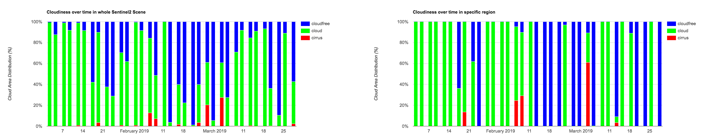 Left: clouds, cirrus and cloudfree areas shown for the whole Sentinel-2 scene - Right: shown for an selected study area.
 Google Earth Engine Javascript Code Editor
Complete Script
This link opens a copy of the script in the Javascript Code Editor, or simply copy & paste the code from below.
// Javascript
var cloudBitMask = 1 << 10;
print(cloudBitMask);
var cirrusBitMask = 1 << 11;
print(cirrusBitMask);
var geometry = ee.Geometry.Polygon(
[[[10.688618863192767, 47.60024343489247],
[10.688618863192767, 47.53723691957702],
[10.776509488192767, 47.53723691957702],
[10.776509488192767, 47.60024343489247]]], null, false);
var region = ee.FeatureCollection([ee.Feature(geometry, {label: 'Valley region'})]);
var addValues = function(image) {
var cloud = image.eq(cloudBitMask).rename('cloud');
var cirrus = image.eq(cirrusBitMask).rename('cirrus');
var cloudfree = image.eq(0).rename('cloudfree');
return image.addBands([cloud,cirrus,cloudfree]);
};
var dataset = ee.ImageCollection('COPERNICUS/S2_SR')
.filterBounds(region)
.filterDate('2019-01-01', '2019-03-30')
.select('QA60')
.map(addValues)
.select(['cloud','cirrus','cloudfree']);
print(dataset)
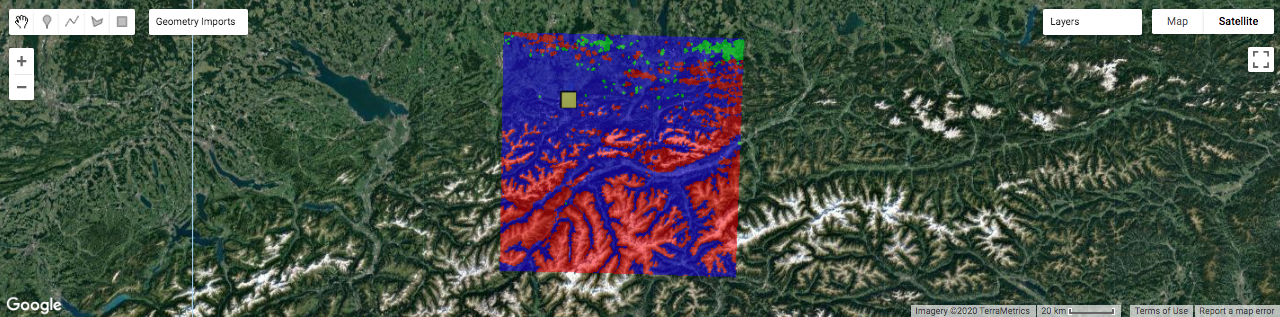
Map.addLayer(dataset, {}, 'Whole Scene Cloudiness', true, 0.5);
var geometry = dataset.first().geometry().buffer(-1000);
var tempTimeSeries_wholeImage = ui.Chart.image.series(
dataset, geometry, ee.Reducer.sum(), 60, 'system:time_start')
.setChartType('ColumnChart')
.setOptions({
isStacked: 'percent',
title: 'Cloudiness over time in whole Sentinel2 Scene',
vAxis: {title: 'Cloud Area Distribution (%)'},
lineWidth: 1,
pointSize: 4,
series: {
0: {color: 'FF0000'},
1: {color: '00FF00'},
2: {color: '0000FF'}
}});
print(tempTimeSeries_wholeImage);
var tempTimeSeries = ui.Chart.image.series(
dataset, region, ee.Reducer.sum(), 60, 'system:time_start')
.setChartType('ColumnChart')
.setOptions({
isStacked: 'percent',
title: 'Cloudiness over time in specific region',
vAxis: {title: 'Cloud Area Distribution (%)'},
lineWidth: 1,
pointSize: 4,
series: {
0: {color: 'FF0000'},
1: {color: '00FF00'},
2: {color: '0000FF'}
}});
print(tempTimeSeries);
Map.addLayer(region,{}, 'Valley region');
Map.centerObject(region,8);
Map.setOptions('SATELLITE')Bottom Line
If you have any questions, suggestions or spotted a mistake, please use the comment function at the bottom of this page.
Previous blog posts are available within the blog archive. Feel free to connect or follow me on Twitter - @Mixed_Pixels.