
This Landsat project would cost...
Many of us read Gabriel Popkin’s nature news article (Popkin 2018) at the end of April this year. Among other things, it stated that officials at the Department of the Interior asked a committee of external advisers to study whether Landsat’s costs could be recovered from users.
Meaning, they are considering whether to charge for access to two widely used sources of remote-sensing imagery:
- the Landsat satellites operated by the US Geological Survey (USGS) and
- an aerial-survey programme run by the Department of Agriculture (USDA).
The US government is considering whether to charge for access to two widely used sources of remote-sensing imagery. https://t.co/R4iNTbRC39
— nature (@Nature) April 24, 2018
The outcry and lack of understanding was, and still is, enormous in the social media world. Scientists from many different fields have started to put a price tag on their used data. Many give the hint that their research would be impossible, because unpayable, without the open Landsat data archive.
Here are just two of the many examples from Twitter:
Landsat data used to be ~$600/scene.
— Joshua Stevens (@jscarto) April 26, 2018
A recent mosaic of mine used > 2300 scenes of data. In the past I'd owe $1.4M. That was for a single map; a day's work.
Technology has far outpaced the notion of paying for scenes. It's simply unimaginable.https://t.co/kEZgULojtT
Landsat imagery for my current project would have cost $20,516,400 at the previous $600/scene fee. No one would/could pay that. Grateful for free Landsat to study how large regions change over multiple decades! Vital for understanding how to manage water resources to grow food.
— Jillian Deines (@JillDeines) June 8, 2018
Motivation
Tyler Erickson and Tim Assal responded to Jillian Deines tweet and made me wonder how difficult it might be to estimate the Landsat data costs within the Google Earth Engine.
Sounds like a good #eeus18 hackathon idea: create a tool for estimating the cost of Landsat (or other imagery) analyzed, if it wasn't freely available.
Right on Jillian! The USGS is currently trying to better estimate the value of #Landsat. We should all do this back of the envelope calculation as well! @USGSLandsat @NASA_Landsat
A quick look at the hackathon list of Google Earth Engine User Summit 2018 in Dublin shows that the proposed Landsat cost estimation hackathon didn’t happen.
However, I think the idea is great and I made a first serve. So here is my example script to estimate the cost of Landsat (if it wasn’t freely available) for the city of Berlin (Germany) between 1984 and 2018 from January til December with a 25% cloud threshold.
Please let me know if you have discovered errors or have suggestions for improvement ;-).
Workflow
Parameter Setup
The user only has to provide 6 pieces of information. The study area (1), the beginning and end of the study period in year (2,3) and month (4,5), as well as a cloud threshold (6) (only a few buy cloudy scenes).
// Javascript

var aoi = geometry;

// #### Parameter Setup ####

var startYear      = 1984;  // what year do you want to start
var endYear        = 2018;  // what year do you want to end
var startMonth     = 1;     // which month do you want to start
var endMonth       = 12;    // which month do you want to end
var max_CloudCover = 25;    // cloud cover threshold, values above are filtered out
Add Landsat WRS-2 grids
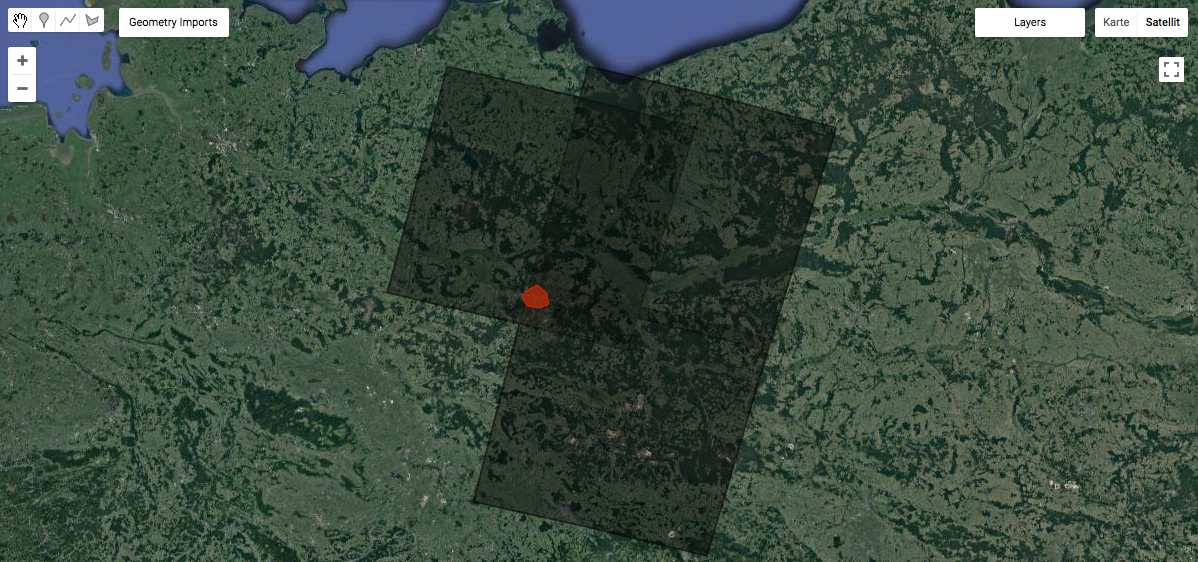 Example geometry: Berlin is covered by three Landsat WRS-2 grids.
To see how many Landsat grids are covering the study area we filter the Worldwide Reference System 2 (WRS2) grid and add it to the map.
// Javascript

var wrs2_descending = ee.FeatureCollection("users/gaertnerp/Blog/WRS2_descending");
var wrs2_filtered   = wrs2_descending.filterBounds(aoi); // filter footprint to aoi

Map.addLayer(wrs2_filtered, {},'WRS2', true, 0.7);  // add layer to map
Map.centerObject(wrs2_filtered, 6);            // center map to footprint
Map.setOptions('SATELLITE')
Create LookUps and Helper Functions
I got the idea with the lookups and helper functions while browsing through the Global Surface Water Tutorial and used it directly, when appropriate.
// Javascript

// # Create a dictionary for looking up sensor names.
var lookup_names = ee.Dictionary.fromLists(
  ['LANDSAT_4', 'LANDSAT_5', 'LANDSAT_7', 'LANDSAT_8'],
  ['LANDSAT 4', 'LANDSAT 5', 'LANDSAT 7', 'LANDSAT 8']
  );

// # Create a dictionary for looking up colors.
var lookup_palette = ee.Dictionary.fromLists(
  ['LANDSAT_4', 'LANDSAT_5', 'LANDSAT_7', 'LANDSAT_8'],
  ['1f78b4', 'a6cee3', 'b2df8a', '33a02c']
  );

function createPieChartSliceDictionary(fc) {
  return ee.List(fc.aggregate_array("class_palette"))
    .map(function(p) { return {'color': p}; }).getInfo();
}
Load Image Collections and add costs
I am assuming that the user uses all available Landsat sensors. If this is not the case, you must comment out lines in the appropriate places (i.e. remove .merge(lt5) if you didn’t use the sensor). Reminder to my future self: There is room for improvement.
My Landsat cost estimates are based on the data from the article Opening the archive: How free data has enabled the science and monitoring promise of Landsat, for more information see (Wulder et al. 2012). There it mentioned in section 3.1
Until the adoption of the open access data policy in 2008, there was always a cost associated with ordering Landsat imagery, and this situation became even more onerous during the commercialization era of the Landsat Program, when copyright restrictions (which were later lifted in 1999) were layered on top of high prices. Costs for an individual photographic image varied from $20 (1972–1978) to $200 (1979–1982) for MSS digital data; digital data ranged from approximately $3000 to $4000 for TM data (1983–1998), and $600 for ETM+ data (1999–2008).
The other day Mike Wulder tweeted again on the subject and added the following valuable information:
For your "This Landsat project would cost..." tweet, it depends on era. Image cost varied over time & mission operations mode (commercial or not). TM data, 1983-1998: up to $4000, $2500 at time of #Landsat-7 launch. ETM+ data, 1999-2008: $600 Post-2008: $0
Landsat image prices as basis for project cost calculation
- I excluded MSS data (Landsat-1, Landsat-2 and Landsat-3)
- For Landsat-4 data, I have taken the lower value of the mentioned range ($3.000 per image)
- For Landsat-5 data, I used $3.000 dollar per image until the year 1998, from 1999 onwards decreased the cost to $2.500 per image
For Landsat-7 & Landsat-8 data, I used the mentioned $600 per image until today, asuming Landsat wasn’t freely available.
// Javascript

// #### IMAGE_COLLECTION FUNCTIONS ####

var getSRcollection = function(startYear, endYear, startMonth, endMonth, sensor, aoi, cost_high, cost_low){

var srCollection = ee.ImageCollection('LANDSAT/'+ sensor + '/C01/T1_SR')
.filterBounds(aoi)
.filterMetadata('CLOUD_COVER', 'not_greater_than', max_CloudCover)
.filter(ee.Filter.calendarRange(startYear,endYear,'year'))
.filter(ee.Filter.calendarRange(startMonth,endMonth,'month'))
.map(function(image) {
var year  = image.date().format("Y"); // get the acquisition year
return image.set('year', ee.Number.parse(year));
})
.map(function(image) {
return ee.Algorithms.If(ee.Number(image.get('year')).gt(1998),
                      image.set('cost', cost_low),
                      image.set('cost', cost_high));

});

return srCollection;

};

var getCombinedSRcollection = function(startYear,endYear, startMonth, endMonth, aoi) {

// ### LANDSAT/LT04/C01/T1_SR ### Aug 22, 1982 - Dec 14, 1993 ###
var lt4 = getSRcollection(startYear,endYear, startMonth, endMonth, 'LT04', aoi, 3000, 3000);

// ### LANDSAT/LT05/C01/T1_SR ### Jan 01, 1984 - May 05, 2012 ###
var lt5 = getSRcollection(startYear,endYear, startMonth, endMonth, 'LT05', aoi, 3000, 2500);

// ### LANDSAT/LE07/C01/T1_SR ### Jan 1, 1999 - open          ###
var le7 = getSRcollection(startYear,endYear, startMonth, endMonth, 'LE07', aoi, 600, 600);

// ### LANDSAT/LC08/C01/T1_SR ### Apr 11, 2013 - Jun 13, 2018 ###
var lc8 = getSRcollection(startYear,endYear, startMonth, endMonth, 'LC08', aoi, 600, 600);

// ### merge the individual sensor collections into one imageCollection object
var mergedCollection = ee.ImageCollection(lt4.merge(lt5).merge(le7).merge(lc8));

return mergedCollection;  // ### return the Imagecollection

};

var LIC = getCombinedSRcollection(startYear,endYear, startMonth, endMonth, aoi);
Calculate Total Landsat Costs
Example Berlin: This Landsat project would have cost 1217700.0 US Dollar($).
// Javascript

// # Get Properties
var featureCollection = ee.FeatureCollection(LIC).select(['year','SATELLITE','cost']);
// ### print(featureCollection)


// # Compute the total project costs
var totalCost = featureCollection.reduceColumns({
  reducer: ee.Reducer.sum(),
  selectors: ['cost'],
});

print(ee.String('This Landsat project would have\ncost ').cat(totalCost.get('sum')).cat(' US Dollar($).'));
Calculate cost allocation per Landsat sensor group
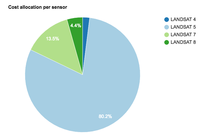 Example Berlin: Landsat sensor allocation between 1984 - 2018.
Here the costs for each Landsat sensor type are calculated individually. Landsat 4 & 5 were much more expensive than e.g. Landsat 7. The final result is displayed as a PieChart.
// Javascript

// # Cost allocation per sensor grouped.
var cost_grouped = featureCollection.reduceColumns({
  selectors: ['cost', 'SATELLITE'],
  reducer: ee.Reducer.sum().group({
     groupField: 1,
     groupName: 'SATELLITE'
    })
});


//# Get the list of groups from the reducer's dictionary.
var cost_grouped_List = ee.List(cost_grouped.get('groups'));


// # Create a feature for each sensor that includes costs.
function createFeature(group_stats) {
  group_stats = ee.Dictionary(group_stats);
  var class_nbr = group_stats.get('SATELLITE');
  var result = {
      class_number: class_nbr,
      sensor_name: lookup_names.get(class_nbr),
      class_palette: lookup_palette.get(class_nbr),
      cost_dollar: group_stats.get('sum')
  };
  return ee.Feature(null, result); // Creates a feature without a geometry.
}

var cost_grouped_fc = ee.FeatureCollection(cost_grouped_List.map(createFeature));


// # Add a summary pie chart.
var summary_pie_chart = ui.Chart.feature.byFeature({
    features: cost_grouped_fc,
    xProperty: 'sensor_name',
    yProperties: 'cost_dollar'
  })
  .setChartType('PieChart')
  .setOptions({
    title: 'Cost allocation per sensor',
    slices: createPieChartSliceDictionary(cost_grouped_fc)
  });

print(summary_pie_chart);
Calculate Landsat cost distribution by year and sensor
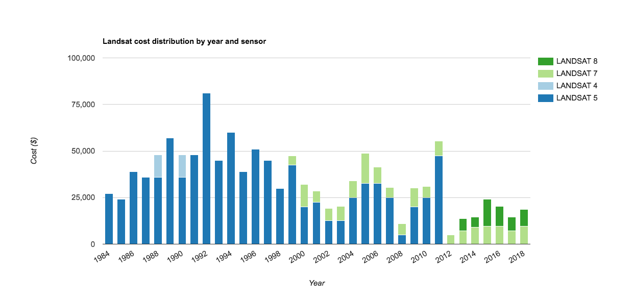 Example Berlin: Landsat cost distribution between 1984 - 2018 (Jan-Dez / 25% clouds).
Last but not least, here I devided the Landsat costs by year and sensor. In order to use the reduceColumns reducer I combined the year and sensor to year-SATELLITE (i.e. 2010-LANDSAT_5), added the costs for each year-SATELLITE group and split the string back into year and SATELLITE for the final ColumnChart.
// Javascript


// #Combine YEAR and SATELLITE for group informations
var featureCollection_combo = featureCollection.map(function (feature) {
    var n1 = feature.get(ee.String('year'));
    var n2 = feature.get('SATELLITE');
    var n1_n2 = ee.String(n1).cat('-').cat(n2);
    return feature.set('n1_n2_combined', n1_n2);
});


// #Devide the total project cost by SATELLITE sensor.
var year_sensor_combined = featureCollection_combo.reduceColumns({
  selectors: ['cost', 'n1_n2_combined'],
  reducer: ee.Reducer.sum().group({
     groupField: 1,
     groupName: 'n1_n2_combined'
    })
});

var year_sensor_combined_List = ee.List(year_sensor_combined.get('groups'));


function createFeature2(group_stats) {
  group_stats = ee.Dictionary(group_stats);
  var class_nbr = group_stats.get('n1_n2_combined');
  var class_nbr_list = ee.String(class_nbr).split("-");
  var sensor = class_nbr_list.get(1);
  var result = {
      year: class_nbr_list.get(0),
      sensor_class: sensor,
      sensor_name: lookup_names.get(sensor),
      cost: group_stats.get('sum')
  };
  return ee.Feature(null, result);   // Creates a feature without a geometry.
}
var year_sensor_combined_fc = ee.FeatureCollection(year_sensor_combined_List.map(createFeature2));


var column_Chart = ui.Chart.feature.groups({
  features: year_sensor_combined_fc,
  xProperty: 'year',
  yProperty: 'cost',
  seriesProperty:'sensor_name'})
    .setChartType('ColumnChart')
    .setOptions({
      title: 'Landsat cost distribution by year and sensor',
      hAxis: {
        title: 'Year'},
      vAxis: {
        title: 'Cost ($)'
      },
      lineWidth: 3,
      isStacked: true,
      series:
      {
    0: {color: '1f78b4' },
    1: {color: 'a6cee3'},
    2: {color: 'b2df8a'},
    3: {color: '33a02c'}
}
});

print(column_Chart);
Bottom line
This blog post showed you how to calculate the Landsat project costs if it wasn’t freely available. There is still a lot of room for improvements and I am happy to hear from you if you have suggestions.
Complete Script
The following link opens a copy of the explained script in the Javascript Code Editor.
You can cite this blogpost using: Gärtner, Philipp (2018/06/26) “This Landsat project would cost…”, https://philippgaertner.github.io/2018/06/landsat-cost-estimator/
If you have any questions, suggestions or spotted a mistake, please use the comment function at the bottom of this page.
Previous blog posts are available within the blog archive. Feel free to connect or follow me on Twitter - @Mixed_Pixels.
References
Popkin, Gabriel. 2018. “US Government Considers Charging for Popular Earth-Observing Data.”
Wulder, Michael A, Jeffrey G Masek, Warren B Cohen, Thomas R Loveland, and Curtis E Woodcock. 2012. “Opening the Archive: How Free Data Has Enabled the Science and Monitoring Promise of Landsat.” Remote Sensing of Environment 122. Elsevier: 2–10.