
How to arrange a raster image stack for the use with BFAST in R
The goal of this blog post is to arrange a irregularly (with varying time intervals) spaced raster stack from Landsat into a regular time series to be used in the Breaks For Additive Season and Trend (bfast) package and function.
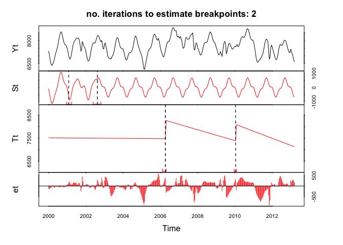 BFAST plot generated with a time series of aggregated bi-weekly NDVI values.
Objective
During the process we impute missing data (NA’s) either:
- linearly with
na.approxfrom thezoopackage, and/or - periodic decomposition with
na.interpfrom theforecastpackage.
We first create a regular daily time series and from that we aggregate the time series with the following frequencies:
- daily (frequency 365) - the base
- weekly (52)
- fortnightly (26)
- monthly (12)
- quarterly (4)
- yearly (1)
Workflow
Load all necessary libraries
### R

library(zoo)
library(xts)
library(forecast)
library(seas)
library(bfast)
library(devtools)
install_github('loicdtx/bfastSpatial')
library(bfastSpatial)  # added 5/2/2019
library(lubridate)
library(ggplot2)
Load the data and select one example pixel
### R

# load data
data(tura)

# get the image dates
dates <- getZ(tura)

selected_pixel <- 90

# number of valid values in TS
nbr.NA <- sum(!is.na( !as.vector(tura[selected_pixel])))

# create a regular time series object by combining data and date information
(s <- bfastts(as.vector(tura[selected_pixel]), dates, type = c("irregular")))

## Time Series:
## Start = c(1984, 157)
## End = c(2013, 101)
## Frequency = 365
##     [1]   NA   NA   NA   NA   NA   NA   NA   NA   NA   NA   NA   NA   NA
##    [14]   NA   NA   NA   NA   NA   NA   NA   NA   NA   NA   NA   NA   NA
##    [27]   NA   NA   NA   NA   NA   NA   NA   NA   NA   NA   NA   NA   NA
##    [40]   NA   NA   NA   NA   NA   NA   NA   NA   NA   NA   NA   NA   NA
##    [53]   NA   NA   NA   NA   NA   NA   NA   NA   NA   NA   NA   NA   NA
##    [66]   NA   NA   NA   NA   NA   NA   NA   NA   NA   NA   NA   NA   NA
##    [79]   NA   NA   NA   NA   NA   NA   NA   NA   NA   NA   NA   NA   NA
##    [92]   NA   NA   NA   NA   NA   NA   NA   NA   NA   NA   NA   NA   NA
##   [105]   NA   NA   NA   NA   NA   NA   NA   NA   NA   NA   NA   NA   NA
##   [118]   NA   NA   NA   NA   NA   NA   NA   NA   NA   NA   NA 7388   NA
##   [131]   NA   NA   NA   NA   NA   NA   NA   NA   NA   NA   NA   NA   NA
##   [144]   NA   NA   NA   NA   NA   NA   NA   NA   NA   NA   NA   NA   NA
##   [157]   NA   NA   NA   NA 5886   NA   NA   NA   NA   NA   NA   NA   NA
##   [170]   NA   NA   NA   NA   NA   NA   NA   NA   NA   NA   NA   NA   NA
##   [183]   NA   NA   NA   NA   NA   NA   NA   NA   NA   NA   NA   NA   NA
##   [196]   NA   NA   NA   NA   NA   NA   NA   NA   NA   NA   NA   NA   NA
##   [209] 6752   NA   NA   NA   NA   NA   NA   NA   NA   NA   NA   NA   NA
##
##   ....
##
## [10375]   NA   NA   NA   NA   NA   NA   NA   NA   NA   NA   NA   NA   NA
## [10388]   NA   NA   NA   NA   NA   NA   NA   NA   NA   NA   NA   NA   NA
## [10401]   NA 7176   NA   NA   NA   NA   NA   NA   NA   NA   NA   NA   NA
## [10414]   NA   NA   NA   NA 7526   NA   NA   NA   NA   NA   NA   NA   NA
## [10427]   NA   NA   NA   NA   NA   NA   NA 7112   NA   NA   NA   NA   NA
## [10440]   NA   NA   NA   NA   NA   NA   NA   NA   NA   NA 7154   NA   NA
## [10453]   NA   NA   NA   NA   NA   NA   NA   NA   NA   NA   NA   NA   NA
## [10466]   NA   NA   NA   NA   NA   NA   NA   NA   NA   NA   NA   NA   NA
## [10479]   NA   NA   NA   NA   NA   NA   NA   NA   NA   NA   NA   NA   NA
## [10492]   NA   NA   NA   NA   NA   NA 6576   NA   NA   NA   NA   NA   NA
## [10505]   NA   NA   NA   NA   NA   NA   NA   NA   NA   NA   NA   NA   NA
## [10518]   NA   NA   NA   NA   NA   NA   NA   NA   NA   NA   NA   NA 7444


# First day of the Time Series
(first.day <- head(date_decimal(as.numeric(time(s))),1))
## [1] "1984-06-05 10:15:27 UTC"

# Last day of the Time Series
(last.day <- tail(date_decimal(as.numeric(time(s))),1))
## [1] "2013-04-10 23:59:59 UTC"
Create Daily Time Series (NA’s - linear, periodic)
Replace NA’s by Linear Interpolation with na.approx from the zoo package
### R

s.d.linear <- round(na.approx(s),0)

# added 3/3/2019
# convert the time series to a data.frame
time.series.to.dataframe <- function(time_series, source) {

  s.df           <- data.frame(as.numeric(time_series))
  colnames(s.df) <- "NDVI"
  s.df$Time      <- as.Date(date_decimal(as.numeric(time(time_series))))
  s.df$Type      <- source
  return(s.df)

}

# create a data.frame
s.d.linear.df <- time.series.to.dataframe(s.d.linear, "Linear Interpolation")
Replace NA’s by periodic stl decomposition with na.interp from the forecast package
### R

s.d.periodic <- round(na.interp(s),0)
Aggregate Time Series from Daily to Weekly
### R

aggregate.daily.to.weekly <- function(daily.ts) {

  dates      <- as.Date(date_decimal(as.numeric(time(daily.ts))))

  xts.daily  <- xts(daily.ts, order.by = dates)

  xts.weekly <- round(xts::apply.weekly(xts.daily, median),0)  # xts

  start(xts.weekly)
  ts.weekly <- ts(data = xts.weekly,
               # define the start and end (Year, Week)
               start = c(as.numeric(format(start(xts.weekly), "%Y")),
                         as.numeric(format(start(xts.weekly), "%W"))),
               end   = c(as.numeric(format(end(xts.weekly), "%Y")),
                         as.numeric(format(end(xts.weekly), "%W"))),
               frequency = 52)

  return(ts.weekly)
}

s.w.linear   <- aggregate.daily.to.weekly(s.d.linear)

start(s.w.linear)
## [1] 1984   41

end(s.w.linear)
## [1] 2013   14


s.w.periodic   <- aggregate.daily.to.weekly(s.d.periodic)

Aggregate Time Series from Daily to Fortnightly
### R

aggregate.daily.to.fortnight <- function(daily.ts) {

  daily.ts.df           <- data.frame(as.numeric(daily.ts))
  colnames(daily.ts.df) <- "NDVI"
  daily.ts.df$date      <- as.Date(date_decimal(as.numeric(time(daily.ts))))

  library(openair)
  ## bi-weekly / fortnightly averages with function timeAverage {openair}
  fortnight      <- timeAverage(daily.ts.df, avg.time = "2 week")
  fortnight$time <- as.Date(fortnight$date)

  fortnight.ts <- ts(fortnight$NDVI,
                     # define the start and end (Year, Week)
               start = c(as.numeric(format(min(fortnight$date), "%Y")),
                         round(yday(min(fortnight$date)) / 14,0)), # DOY / 14
               end   = c(as.numeric(format(max(fortnight$date), "%Y")),
                         round(yday(max(fortnight$date)) / 14,0)), # DOY / 14
                     frequency = 26)

  return(fortnight.ts)
}

s.f.linear   <- aggregate.daily.to.fortnight(s.d.linear)
## Warning: package 'openair' was built under R version 3.4.4

s.f.periodic <- aggregate.daily.to.fortnight(s.d.periodic)

start(s.f.linear)
## [1] 1984   20

end(s.f.linear)
## [1] 2013    6

Aggregate Time Series from Daily to Monthly
### R

aggregate.daily.to.monthly <- function(daily.ts) {

  s.month <- round(aggregate(as.zoo(daily.ts), as.yearmon, median), 0)   # zoo
  s.month <- as.ts(s.month)

  return(s.month)

}

s.m.linear   <- aggregate.daily.to.monthly(s.d.linear)
s.m.periodic <- aggregate.daily.to.monthly(s.d.periodic)

start(s.m.linear)
## [1] 1984   10

end(s.m.linear)
## [1] 2013    4

Aggregate Time Series from Daily to Quarterly
### R

aggregate.daily.to.quarterly <- function(daily.ts) {

  s.qtr <- round(aggregate(as.zoo(daily.ts), as.yearqtr, median), 0)   # zoo
  s.qtr <- as.ts(s.qtr)

  return(s.qtr)

}

s.q.linear   <- aggregate.daily.to.quarterly(s.d.linear)
s.q.periodic <- aggregate.daily.to.quarterly(s.d.periodic)

start(s.q.linear)
## [1] 1984    4

end(s.q.linear)
## [1] 2013    2

Aggregate Time Series from Daily to Yearly Season
The time of summer start and end depends on the location on the globe. The Tura dataset is from Ethopia and we consider June, July and August as their summer season, meaning we consider only these months for our yearly aggragation calculation.
### R

#https://stackoverflow.com/questions/18978256/what-is-the-most-elegant-way-to-calculate-seasonal-means-with-r

aggregate.daily.to.yearly <- function(daily.ts) {

  # create data.frame
  daily.df <- time.series.to.dataframe(daily.ts, "not needed here")

  # add year
  daily.df$year <- format(daily.df$Time, "%Y")

  # add season
  daily.df$seas <- mkseas(x = daily.df, width = "DJF")

  # calculate median per season within each year
  year.df <- aggregate(NDVI ~ seas + year, data = daily.df, median)

  # based on variable values
  year.df.JJA <- year.df[ which(year.df$seas == 'JJA'), ]

  # create ts
  year.ts.JJA <- ts(year.df.JJA$NDVI,
                    start = c(as.numeric(min(year.df.JJA$year)), 1), # freq 1
                    end   = c(as.numeric(max(year.df.JJA$year)), 1), # freq 1
                    frequency = 1)

  return(year.ts.JJA)
}

(s.y.linear   <- aggregate.daily.to.yearly(s.d.linear))
## Time Series:
## Start = 1985
## End = 2012
## Frequency = 1
##  [1] 6088.5 7552.0 7012.5 7633.0 7672.0 7712.0 7751.0 7791.0 7830.0 7870.0
## [11] 7527.0 7739.5 7950.5 8162.0 8373.5 7963.0 8133.5 8080.5 7476.0 7872.0
## [21] 7286.5 8116.5 8298.5 7509.5 7187.0 8227.5 7656.5 7904.0

(s.y.periodic <- aggregate.daily.to.yearly(s.d.periodic))
## Time Series:
## Start = 1984
## End = 2012
## Frequency = 1
##  [1] 7433.0 6914.5 8028.0 7063.5 7367.5 7443.5 7519.5 7595.5 7671.5 7747.5
## [11] 7824.0 7460.0 7645.0 7829.0 8015.0 8200.0 7997.5 8142.5 8008.0 7501.5
## [21] 7715.0 7853.5 8304.0 8161.0 8132.0 7629.5 8409.0 7585.5 7784.5

Focus on a Specific Period
Once you have your data prepared and you would like to work on a specific temporal window you can use the ‘window’ function to cookie cut the period of interest.
For example, use the Fortnight time series and focus on the data from year 2000, onwards.
### R

s.f.periodic.window <- window(x = s.f.periodic,
                     start = c(2000,1),
                     frequency = 26) # Fortnight has a frequency of 26

plot(s.f.periodic.window, ylab = "NDVI")
Testing the aggregated Time Series with BFAST
Here we do a simple test if bfast will accept the created fortnight time series. Lets see…
Yeap … it works beautifully!
### R

fit <- bfast(s.f.periodic.window, h = 10/length(s.f.periodic.window),
             season = "harmonic", breaks = 2, max.iter = 2)

plot(fit)
Bottom line
This blog post showed you how to arrange and aggragate a raster image stack in order to create a regular time series which can be used with the bfast function. If you have any questions, suggestions or spotted a mistake, please use the comment function at the bottom of this page.
You can cite this blogpost using: Gärtner, Philipp (2018/04/16) “How to arrange a raster image stack for the use with BFAST in R”, https://philippgaertner.github.io/2018/04/bfast-preparation/
Previous blog posts are available within the blog archive. Feel free to connect or follow me on Twitter - @Mixed_Pixels.
Data Source
- Tura: The used Tura dataset is provided by the
bfastSpatialpackage. It covers a area in Tura kebele, Kafa Zone, SW Ethiopia. The values are NDVI rescaled by a factor of 10000. Data originate from the Landsat 5 TM and Landsat 7 ETM+ sensors. Original Landsat scene names can be found by typingnames(tura). Dates are also contained in the z-dimensiongetZ(tura).