The blog post shows how the vegetation of two public parks changes seasonally. Multi-temporal satellite images were used to aggregate monthly histograms of vegetation index values. The visualization was inspired by this tweet from Christopher Doyle.

Intra-annual vegetation density changes of two public parks in Berlin, Germany.

Green spaces in the middle of the city

The topic in this blog post is Berlin, the pulsating metropolis everyone is talking about, at least that’s what most Berliner claim. But I won’t write about the club scene nor about hipster migration or the overcrowded, delayed local traffic.

Today, I write about two major parks in Berlins city center and show how their vegetation density changes seasonally over the course of the year. I am writing about the phenology.

Areas of Interest: Tiergarten and Tempelhofer Feld

Tiergarten is a popular inner-city park between the Kanzleramt and the Sony Business Center. About half of the Tiergarten consists of meadows the other half of woodland. The park is 210 ha in size and is among the largest urban gardens of Germany. Only Munich’s Englischer Garten and the Tempelhofer Feld, also in Berlin, are larger.

Now that I’m on it, the second park under investigation is the Tempelhofer Feld. The Tempelhofer Feld is with 355 ha the largest inner-city open space in the world. It is dominated by meadows but has at least 20 hectares of endangered and protected dry sand grassland and 27 hectares of plain oatmeal meadow.

Data generation in Earth Engine

The data basis for the illustration of the seasonal density change in the park vegetation were satellite images. Here, I used all USGS provided images (> 260) of Landsat 8 Collection 1 Tier 1, for each of the two parks, determined the Normalized Difference Vegetation Index (NDVI) and created a monthly NDVI histogram for all cloudless pixels depending on the date of recording and exported the result as .geojson. Very helpful was this page in the GEE Documentation.

In order to run the code you need access to the park polygons. Hereby I share the links to the Tiergarten und Tempelhof shapes, so everybody has read access to the asset and will be able to view und use them in the code editor.

GetData

// Javascript

// This function gets NDVI from a Landsat 8 image.
var addNDVI = function(image) {
  return image.addBands(image.normalizedDifference(['B5', 'B4']));
};

// This function masks cloudy pixels.
var cloudMask = function(image) {
  var clouds = ee.Algorithms.Landsat.simpleCloudScore(image).select(['cloud']);
  return image.updateMask(clouds.lt(25));
};

// Load a Landsat collection, map the NDVI and cloud masking functions over it.
var collection = ee.ImageCollection('LANDSAT/LC08/C01/T1_TOA')
  .filterBounds(Tiergarten.geometry())
  .filter(ee.Filter.calendarRange(12,12, "month")) // only December
  .map(addNDVI)
  .map(cloudMask);

// Reduce the collection to the medan of each pixel and display.
var medianImage = collection.reduce(ee.Reducer.median());

// Reduce the region. The region parameter is the Feature geometry.
var median_Dictionary = medianImage.select(['nd_median']).reduceRegion({
  reducer: ee.Reducer.histogram({minBucketWidth: 0.01}),
  geometry: Tiergarten.geometry(),
  scale: 30,
  bestEffort: true
});

var FC = ee.Dictionary({median_Dictionary:median_Dictionary});

var features  = ee.Feature(null, {FC: FC});
var export_FC = ee.FeatureCollection([features]);

Export.table.toDrive({
  collection: export_FC,
  folder: 'GEE',
  description: 'Tiergarten_12', 
  fileFormat: 'GeoJSON'
});




// This function gets NDVI from a Landsat 8 image.
var addNDVI = function(image) {
  return image.addBands(image.normalizedDifference(['B5', 'B4']));
};

// This function masks cloudy pixels.
var cloudMask = function(image) {
  var clouds = ee.Algorithms.Landsat.simpleCloudScore(image).select(['cloud']);
  return image.updateMask(clouds.lt(25));
};

// Load a Landsat collection, map the NDVI and cloud masking functions over it.
var collection = ee.ImageCollection('LANDSAT/LC08/C01/T1_TOA')
  .filterBounds(Tiergarten.geometry())
  .filter(ee.Filter.calendarRange(12,12, "month")) // only December
  .map(addNDVI)
  .map(cloudMask);

// Reduce the collection to the medan of each pixel and display.
var medianImage = collection.reduce(ee.Reducer.median());

// Reduce the region. The region parameter is the Feature geometry.
var median_Dictionary = medianImage.select(['nd_median']).reduceRegion({
  reducer: ee.Reducer.histogram({minBucketWidth: 0.01}),
  geometry: Tiergarten.geometry(),
  scale: 30,
  bestEffort: true
});

var FC = ee.Dictionary({median_Dictionary:median_Dictionary});

var features  = ee.Feature(null, {FC: FC});
var export_FC = ee.FeatureCollection([features]);

Export.table.toDrive({
  collection: export_FC,
  folder: 'GEE',
  description: 'Tiergarten_12', 
  fileFormat: 'GeoJSON'
});

All available Landsat-8 satellite imagery for Berlin - ESRI Landsat Viewer.

Data preprocessing with R

In the following section I present the steps you have to take to get from an Earth Engine produced .json file to a the animated GIF. The following code chunks are written in R.

Load all necessary libraries

### R

library(needs) # install.packages("needs")
needs(devtools, RJSONIO, ggplot2, tweenr, stringr, plyr, matrixStats, gganimate)

Load the data from the ‘GEE’ folder into a data.frame

### R

file <- list.files("GEE")

dd <- data.frame()

for(i in 1:length(file)) {

  d_json <- RJSONIO::fromJSON(paste("GEE/", file[[i]], sep=""))

  hist        <- d_json$features[[1]]$properties$FC$median_Dictionary$nd_median$histogram
  bucketMeans <- d_json$features[[1]]$properties$FC$median_Dictionary$nd_median$bucketMeans
  df <- data.frame(bucketMeans, hist, file[[i]])
  dd <- rbind(dd, df)
  
}

colnames(dd) <- c("bucketMeans", "hist","i") # rename d.f columns
head(dd, n = 2)

##   bucketMeans hist                 i
## 1 -0.06514288    2 Tempelhof_01.json
## 2 -0.05500000    0 Tempelhof_01.json

dd is the result of the histogram reducer which divided the entire range of image values into a series of intervals—and then counted how many values fall into each interval. bucketMeans represents the bin (intervals) and hist the value count and i is the file name.

Split column `i` and create a `location` and `month` column

### R

a    <- data.frame(str_split(dd$i, "_"))
a    <- t(a)
a    <- data.frame(a)
a$X2 <- str_replace(a$X2, ".json", "")

dd$location <- a$X1               # column location
dd$month    <- as.numeric(a$X2)   # column month
dd$i        <- NULL               # remove original "i" column
dd$hist     <- round(dd$hist, 0)

colnames(dd) <- c("x", "y", "location", "month")
str(dd)

## 'data.frame':	1733 obs. of  4 variables:
##  $ x       : num  -0.0651 -0.055 -0.0439 -0.035 -0.0299 ...
##  $ y       : num  2 0 4 0 2 1 2 2 15 66 ...
##  $ location: Factor w/ 2 levels "Tempelhof","Tiergarten": 1 1 1 1 1 1 1 1 1 1 ...
##  $ month   : num  1 1 1 1 1 1 1 1 1 1 ...


summary(dd)

##        x                 y                location       month       
##  Min.   :-0.1706   Min.   :  0.00   Tempelhof :815   Min.   : 1.000  
##  1st Qu.: 0.1450   1st Qu.:  3.00   Tiergarten:918   1st Qu.: 4.000  
##  Median : 0.3251   Median : 25.00                    Median : 7.000  
##  Mean   : 0.3274   Mean   : 57.09                    Mean   : 6.563  
##  3rd Qu.: 0.5059   3rd Qu.: 70.00                    3rd Qu.: 9.000  
##  Max.   : 0.8316   Max.   :486.00                    Max.   :12.000

Round bin values and create dummy a `data.frame`

To make the visualization easier we need for each month the same amout of bins, so I create a dummy data.frame with all possible value combination between x (bins) and month, starting from -0.2 until 0.9.

### R

dd$x        <- round_any(dd$x, accuracy = 0.01, f = ceiling) 

# 12 (month) * 111 (NDVI value) = 1332 in total (ideal world row numbers) 
combn_NDVI  <- seq(-0.2,0.9, by = 0.01)
combn_month <- seq(1,12    , by = 1)

tempelhof <- tiergarten <- data.frame(month = rep(combn_month, each = length(combn_NDVI)),
                                      x     = rep(combn_NDVI, 12),              
                                      y     = 0) 

tiergarten$location <- "Tiergarten"
tempelhof$location  <- "Tempelhof"

df <- rbind(tiergarten, tempelhof)
dim(df)
## [1] 2664    4

Merge GEE data and the dummy `data.frame`

### R

dat <- merge(x = dd, y = df, by = c("location", "month", "x"), 
                     all.y = T)

dat[is.na(dat)] <- 0     # convert NA's to 0
dat$y.y         <- NULL  # delete uncessesary columns
colnames(dat)   <- c("location", "time" ,"x", "y")

Smooth the curve

### R

dat_temp  <- dat[dat$location == "Tempelhof", ]
dat_tier  <- dat[dat$location == "Tiergarten", ]

do_it <- function(dataset) {
  models <- dlply(dataset, .(time), function(df) loess(y ~ x, data = df, span = 0.1))
  predict(models[[1]])
  
  x <- ldply(models, predict)
  
  library(reshape)
  xx <- melt(x, id = c("time"))
  xx <- xx[order(xx$time),]
  return(xx)
}

xx <- do_it(dat_temp)
dat_temp$y_loess <- round(xx$value, 1)
dat_temp$y_loess[dat_temp$y_loess < 0] <- 0 # remove values beyond zero

####

xx <- do_it(dat_tier)
dat_tier$y_loess <- round(xx$value,1)
dat_tier$y_loess[dat_tier$y_loess < 0] <- 0

tail(dat_tier, n = 2)

##        location time    x y y_loess
## 2663 Tiergarten   12 0.89 0       0
## 2664 Tiergarten   12 0.90 0       0

Add the `ease` and `group` columns for `tweenr`

### R

create_ease_and_group_for_tween <- function(dataset) {

  dataset$ease  <- "linear"
  dataset       <- dataset[order(dataset$x),]
  dataset$group <- rep(1:length(combn_NDVI), each = 12)      
  
  dataset_tween <- tween_elements(data = dataset, time = 'time', group = 'group', 
                                   ease = 'ease', nframes = 111)
  return(dataset_tween)
}

dat_temp_tween <- create_ease_and_group_for_tween(dat_temp)
dat_tier_tween <- create_ease_and_group_for_tween(dat_tier)

dat_tween       <- rbind(dat_temp_tween, dat_tier_tween)
dat_tween$label <- round(dat_tween$time,0)
dat_tween$label <- month.name[dat_tween$label]

dim(dat_tween)

## [1] 24864     8


tail(dat_tween, n = 2)

##          location time    x y y_loess .frame .group    label
## 109761 Tiergarten   12 0.77 0       0    111     98 December
## 110881 Tiergarten   12 0.78 0       0    111     99 December

Calculate a median for every point in time

### R

gg_df <- ddply(dat_tween, .(location, time), mutate,
                          weighted_median = weightedMedian(x,y_loess))

tail(gg_df, n = 2)

##         location time    x y y_loess .frame .group    label
## 24863 Tiergarten   12 0.77 0       0    111     98 December
## 24864 Tiergarten   12 0.78 0       0    111     99 December
##       weighted_median
## 24863       0.2403083
## 24864       0.2403083

Plot the graph with ggplot + tweenr

Create the `ggplot` + `tweenr` histogram animation for the Tempelhofer Feld and the Tiergarten

### R

p <- ggplot(data = gg_df) + 
  # add label for time (month)
  geom_text(data = gg_df[which(gg_df$location == 'Tiergarten'),],
          aes(x = 0.42, y = 400, frame = .frame, label = label), 
          fontface = "bold", size = 20, color = "#d9d9d9") + 
  # add median point for Tempelhof
  geom_segment(data = gg_df[which(gg_df$location == 'Tempelhof'),],
               aes(x = weighted_median, y = 0, xend = weighted_median, yend = 490,
                   frame = .frame), size = 1, colour = "#737373") + 
  # add label for time (month) 
  geom_text(data = gg_df[which(gg_df$location == 'Tempelhof'),],
          aes(x = weighted_median, y = 540, frame = .frame, 
              label = "Median\nTempelhofer Feld"),size = 5, colour = "#737373") + 
  # add median point for Tiergarten
  geom_segment(data = gg_df[which(gg_df$location == 'Tiergarten'),],
               aes(x = weighted_median, y = 0, xend = weighted_median, yend = 490,
                   frame = .frame), colour = "#737373", size = 1) + 
  # add median text for Tiergarten
  geom_text(data = gg_df[which(gg_df$location == 'Tiergarten'),],
          aes(x = weighted_median, y = 540, frame = .frame, 
              label = "Median\nTiergarten"),size = 5, colour = "#737373") + 
  # add NDVI ribbon for Tempelhof
  geom_ribbon(data = gg_df[which(gg_df$location == 'Tempelhof'),], 
              aes(x = x, ymin = 0, ymax = y_loess, fill = "#2CA02C",frame = .frame),
              alpha = 0.6) +
  # add NDVI ribbon for Tiergarten
  geom_ribbon(data = gg_df[which(gg_df$location == 'Tiergarten'),],
              aes(x = x, ymin = 0, ymax = y_loess, frame = .frame, fill = "#FF7F0E"),
              alpha = 0.6) +
  labs(x = "", y = "") + theme_bw() + xlim(-0.1, 0.9) + ylim(0, 600) + 
  scale_fill_manual(values   = c("#2CA02C", "#FF7F0E"), 
                      labels = c("Tempelhofer Feld   ", "Tiergarten")) + 
  scale_x_continuous(breaks = c(0, 0.25, 0.375, 0.5, 0.75), 
                     labels = c("Low", "", "Medium","", "High")) + 
  theme(legend.position   = "bottom", 
        legend.title      = element_blank(),
         axis.text.x      = element_text(size = 15, colour ="#737373"),
         axis.line.y      = element_blank(), 
         axis.line.x      = element_blank(),
         panel.border     = element_blank(),
         axis.text.y      = element_blank(),
         axis.ticks       = element_blank(),
         panel.grid.major = element_blank(),
         panel.grid.minor = element_blank(),
         panel.background = element_blank(),
         strip.background = element_blank(),
         legend.text      = element_text(size = 15, colour ="#737373", face = "bold"),
         legend.key.size  = unit(1.5, 'cm')) + 
  guides(fill = guide_legend(keywidth = 3.5, keyheight = 1.5))
        
  
animation::ani.options(interval = 1/5)
gganimate(p, 'Histogram_Tiergarten_Tempelhof_animated_0_01.gif', 
          title_frame = F, 
          ani.width = 800, 
          ani.height = 400)

## Scale for 'x' is already present. Adding another scale for 'x', which
## will replace the existing scale.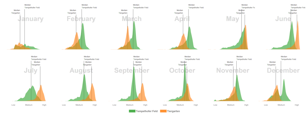

Intra-annual vegetation density changes of two public parks in Berlin, Germany

Intra-annual vegetation density changes

Unfortunately I don’t have any field data to validate my comments on the graphic here, so please use caution.

The median NDVI values of the Tempelhofer Feld are higher in the winter and spring months than in the Tiergarten. The process of photosynthesis in the sprouts is reduced to a minimum. However, the sprouts of the grasses grow actively at temperatures > 10 °C and we’ve had a few days over the last few years far above these temperatures. Furthermore, the Tiergarten is stocked +/- 50% with deciduous trees and those lose their leaves in autumn. The autumn leaf also no longer forms a new chlorophyll and thus gradually loses its green colour, the NDVI decreases.
In June, all the trees in the Tiergarten have turned out their leaves and the meadows grow superbly on the Tempelhofer Feld. Nevertheless, the multi-layered canopy roof in the Tiergarten usually has a higher leaf-area and canopy density which have generaly a positive relationship with the NDVI. In consequence, the Tiergarten has higher NDVI values in the summer months.
In January there are significantly fewer values in the histogram than in summer. The reason for this is that the cloud pixels were filtered out during the histogram calculation.

Bottom line

You can cite this blogpost using: Gärtner, Philipp (2017/11/07) “Intra-annual vegetation density changes of two public parks in Berlin, Germany”, https://philippgaertner.github.io/2017/10/tempelhof_tiergarten/

If you have any questions, suggestions or spotted a mistake, please use the comment function at the bottom of this page.

Previous blog posts are available within the blog archive. Feel free to connect or follow me on Twitter - @Mixed_Pixels.

Data Source

Park Polygons: The park polygons come from Michael Hörz berlin-shapes github repository.
Satellite Data: The Landsat 8 Collection 1 Tier 1 calibrated top-of-atmosphere reflectance datat are provided by the USGS and made available by google as ImageCollection.