
In this tutorial I focus on the availability of Landsat Level-1 data products (calibrated top-of-atmosphere reflectance, orthorectified scenes only) recorded by
- the Thematic Mapper ™ sensor onboard Landsat 4 and 5,
- the Enhanced Thematic Mapper Plus (ETM+) sensor onboard the Landsat 7 satellite,
- the Operational Land Imager (OLI) sensor onboard the Landsat 8 satellite.
In order to use the tutorial code you would need to sign up to get access to Google’s Earth Engine. Once this is done, you will see that the tutorial is divided into sections. Each section provides Javascript code which builds up gradually to the final product.
Table of Contents
 The End Product - A Metadata Application
Application Initiation
In order to get the Application initialized, you have to open the script in the Code Editor and run the entire code once with Run. Now, the application is responding and does a couple of things in the background.
1. Drop-Down Country Selection
- load a FeatureCollection from the Countries of the world,
- load a FeatureCollection from the WRS-2 grids,
- get a list of Country names from the country boundary FeatureCollection,
- create a drop-down menu with the list of Country names as selection option,
- add the drop-down menu widget to the map
For the User begins the Metadata Application actually now with the selection of a country by means of the freshly created drop-down selection menu. Let’s assume the user selected Germany (it could also be any other country). The selection starts the redraw function, the main workhorse of the application, which does the following things:
- center the map to the geographical boundary of Germany,
- add a layer (purple colour) with the outline of Germany to the map
The script for these actions would look like this (Open in Code Editor).
// Load country boundaries
var countries = ee.FeatureCollection("USDOS/LSIB_SIMPLE/2017");
// Load Footprint of Landsat WRS2
var wrs2_descending = ee.FeatureCollection("users/gaertnerp/Blog/WRS2_descending");
function redraw(key){
var selectedCountry = ee.Feature(countries.filter(ee.Filter.eq('country_na', key)).first());
Map.centerObject(selectedCountry);
var selectedCountry_Strg = ee.String(selectedCountry.get('country_na'));
// Show country
var layer0 = ui.Map.Layer(selectedCountry, {color:'purple'}, 'Selected country');
Map.layers().set(0, layer0);
}
// get sorted country names
var names = countries.aggregate_array('country_na').sort();
// initialize combo-box and fire up the redraw function
var select = ui.Select({items: names.getInfo(), onChange: redraw });
select.setPlaceholder('Choose a country ...');
// Add the drop-down 'select' widget to the map
Map.add(select);
Map.setOptions("SATELLITE");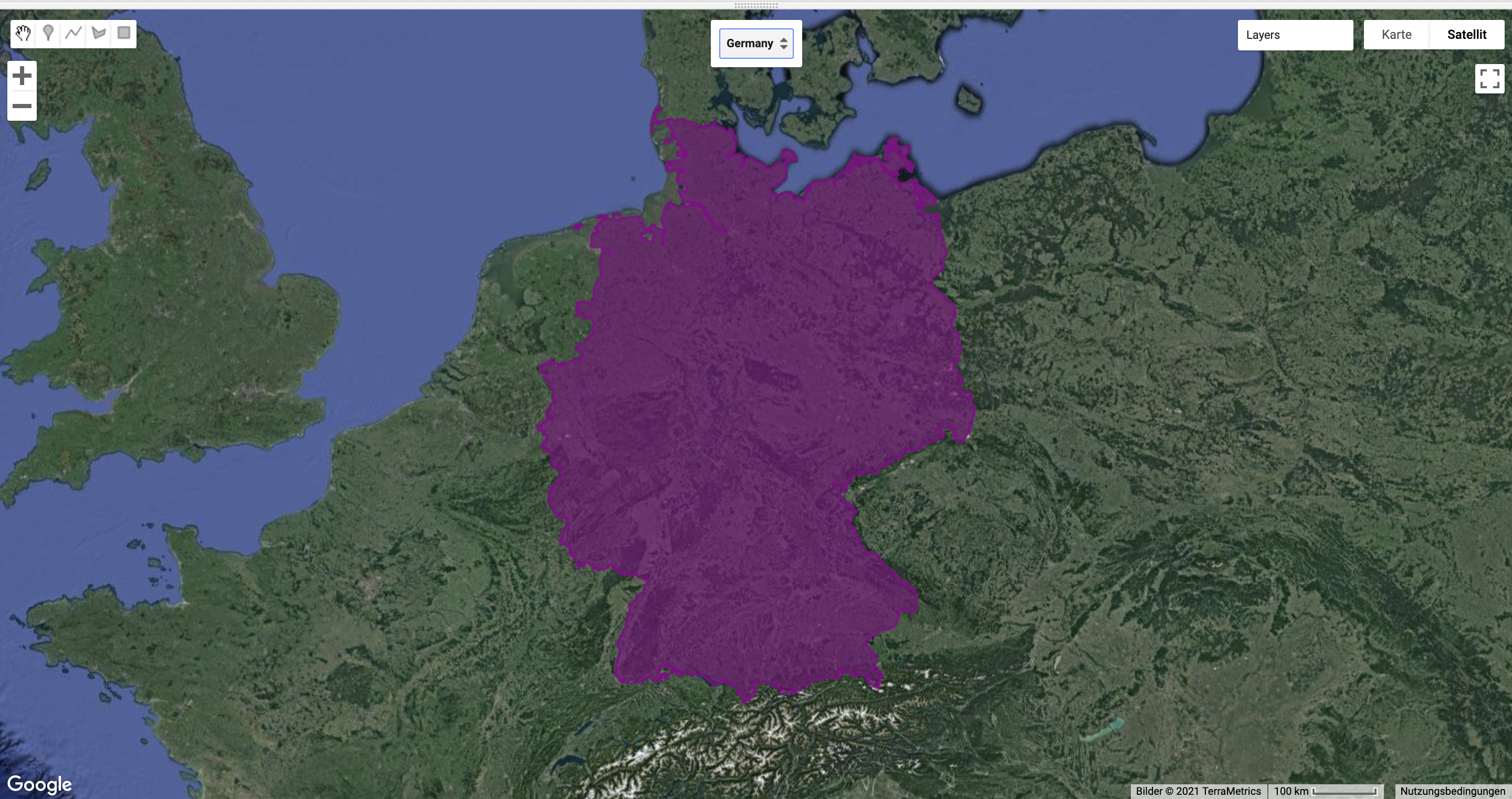 Outline of selected country - Germany
2. Adding Selected Country Borders
In the next step, we add the Landsat WRS 2 Descending Path Row boundaries to the redraw function (Open in Code Editor).
function redraw(key){
// ... continuing the redraw function ........
// show WRS2 footprint
var wrs2_filtered = wrs2_descending.filterBounds(selectedCountry.geometry());
var layer1 = ui.Map.Layer(wrs2_filtered, {color: 'grey', opacity: 0.1 }, 'WRS2 filtered');
Map.layers().set(1, layer1);
Map.setZoom(6);
// ...........
}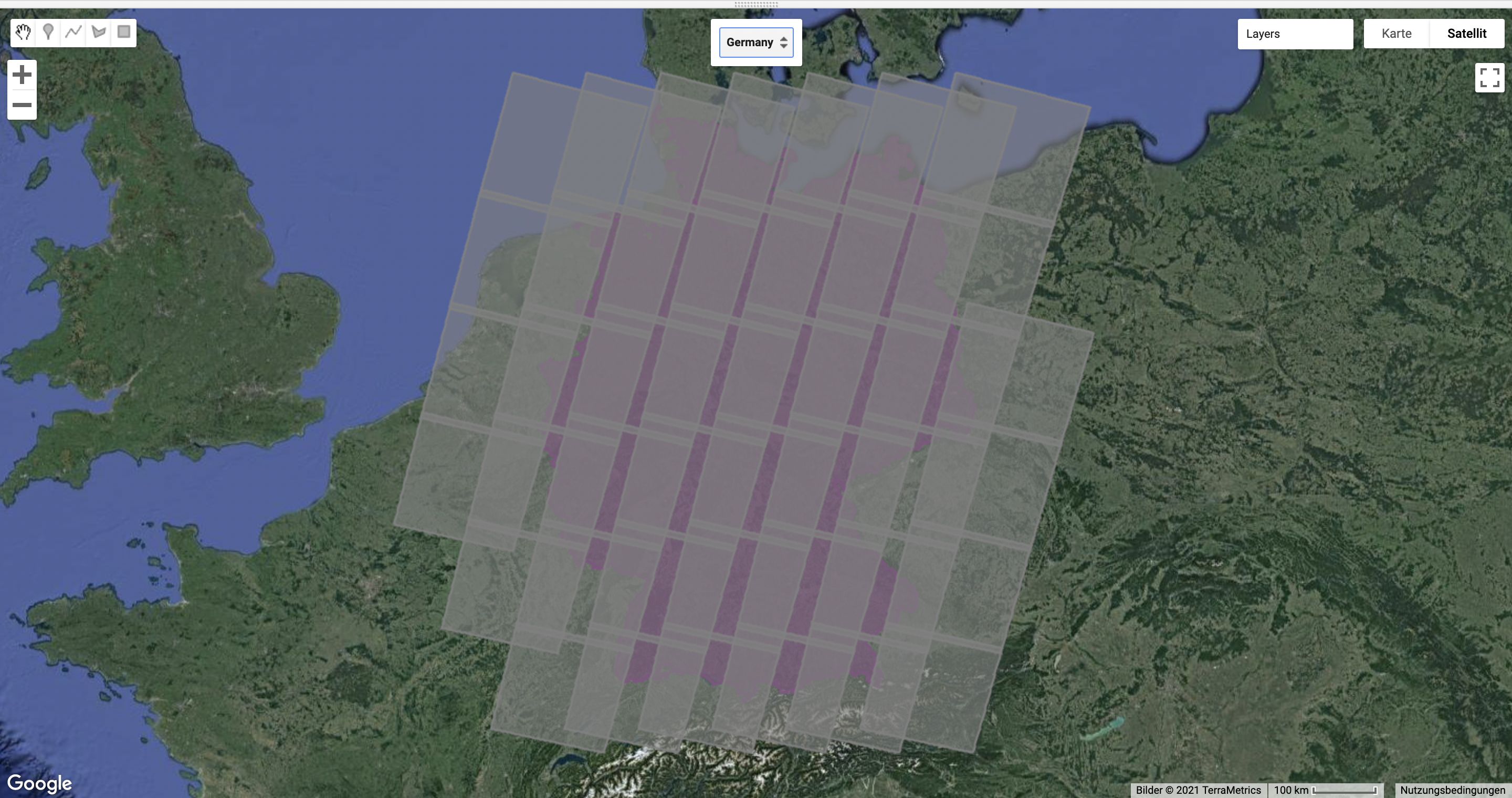 Filtered Landsat WRS 2 descending path row boundaries for Germany
3. Load and Filter Landsat ImageCollections
In order to get information about Landsat 4, 5, 7 and 8 Landsat Level-1 data, we load these as individual ImageCollections and merge them together to a giant dataset.
var l4_coll = ee.ImageCollection("LANDSAT/LT4_L1T_TOA");  //Aug 22, 1982 - Dec 14, 1993
var l5_coll = ee.ImageCollection('LANDSAT/LT5_L1T_TOA');  //Jan 1, 1984 - May 5, 2012
var l7_coll = ee.ImageCollection('LANDSAT/LE7_L1T_TOA');  //Jan 1, 1999 - ongoing
var l8_coll = ee.ImageCollection('LANDSAT/LC8_L1T_TOA');  //Apr 11, 2013 - ongoing

var merged_collection = ee.ImageCollection(l4_coll.merge(l5_coll).merge(l7_coll).merge(l8_coll));
Now, we continue with the redraw function by
- filtering the Landsat ImageCollection with the selected country polygon,
- get for each image the year of the acquisition,
- get the ‘CLOUD_COVER’ metadata property for each image,
- add these metadata properties to the ImageCollection and
- count the number of images within the ImageCollection.
  // ... continue the redraw function ........

  // filter the ImageCollection with the boundary of the selected country
  var iC = merged_collection.filterBounds(selectedCountry.geometry())
                            .filter(ee.Filter.notNull(ee.List(['CLOUD_COVER'])));

  iC = iC.map(function(img){
    var year  = img.date().format("Y"); // get the acquisition year
    var CC    = img.get('CLOUD_COVER');
    return img.set('year', ee.Number.parse(year)).set('clouds', ee.Number.parse(CC)); //
  });

  var iC_FC = ee.FeatureCollection(iC);
  var iC_FC_size = iC_FC.size();

  // ...........
4. Draw Histograms
Chart: Landsat Mission 4-8 - GEE image availability
Now, we can draw two histogram charts which will be plotted in the lower right corner Panel area. The first chart shows the image availability, with time on the x-axis and Image count on the y-axis.
// ... continue the redraw function ........

var options1 = {
    title: 'Landsat Mission 4-8 - GEE image availability',
    hAxis: {title: 'Year'},
    vAxis: {title: 'Image count'},
    colors: ['red']
};

var histogram = ui.Chart.feature.histogram({
    features: iC_FC,
    property: 'year',
    minBucketWidth: 1
}).setOptions(options1);

panel.widgets().set(0, histogram);

// ...........

Chart: Landsat cloud cover
The second chart shows the Cloud cover % for all images recorded over Germany. The chart has a 5% Cloud cover bin width on the x-axis and shows again the Image count on the y-axis.
// ... continue the redraw function ........

var options2 = {
    title: 'Landsat cloud cover',
    hAxis: {title: '% Cloud Cover'},
    vAxis: {title: 'Image count'},
    colors: ['orange']
};

var histogram_CC = ui.Chart.feature.histogram({
    features: iC_FC,
    property: 'clouds',
    minBucketWidth: 5
}).setOptions(options2);

panel.widgets().set(1, histogram_CC);

// ...........

Add Info Text
With the information on the Country name (Germany) the amount of WRS-2 grids (43) as well as the total number of recorded Landsat imagery (16003), I added a small informative info-text to the Panel.
// ... continue the redraw function ........

var iscoveredby = " is covered by ";
var wrs2_filtered_size = wrs2_filtered.size();
var LandsatWRSgridsIntotalwere = " Landsat WRS-2 grids. During the lifetime of Landsat Mission 4-8 were ";
var text = " images collected. Their spatial distribution is shown in the map (red circles), the temporal distribution is shown in the first chart.";
var text2 = " The relative average cloud cover for each WRS-2 is shown in the map (orange circles), while the 2nd chart shows a histogram of the overall percentage cloud cover."
var info_text = ee.String(selectedCountry_Strg).cat(iscoveredby).cat(wrs2_filtered_size)
.cat(LandsatWRSgridsIntotalwere).cat(iC_FC_size).cat(text).cat(text2);

info_text.evaluate(function(result) {
    panel.widgets().set(2, ui.Label(result));
});

// ...........
Germany is covered by 43 Landsat WRS-2 grids. During the lifetime of Landsat Mission 4-8 were 16003 images collected. Their spatial distribution is shown in the map (red circles), the temporal distribution is shown in the first chart. The relative average cloud cover for each WRS-2 is shown in the map (orange circles), while the 2nd chart shows a histogram of the overall percentage cloud cover.
Add for each WRS-2 grid individually sized centroid points
Here comes the most interesting part of the tutorial. The idea is, to show in the centre of each WRS-2 grid a circle, which size is dependent on the amount of the recorded images.
- a small circle would mean, just a few images were recorded, while
- a bigger circle means, here are more images available.
Get the Centroid
The getCentroid function is used to
- get the centre point (centroid) of each WRS-2 grid geometry and
keep the Row and Path properties
// ... continue the redraw function ........

// create centroids
var centroids = wrs2_filtered.map(getCentroid);
var fC        = centroids.map(addField);

// ...........
// begin - getCentroid var getCentroid = function(feature) { // Keep this list of properties. var keepProperties = ['PATH', 'ROW']; // Get the centroid of the feature's geometry. var centroid = feature.geometry().centroid(); // Return a new Feature, copying properties from the old Feature. return ee.Feature(centroid).copyProperties(feature, keepProperties); }; // end - getCentroid
Match image availibility and cloud cover with circle size

Finally, the addField function is used to
- iterate over the merged ImageCollection
- filter each Path/Row pair,
- calculate the average Cloud_Cover (lets assume 50%)
- count the images (lets assume n = 400 images),
- now I create a red circle with 40km radius (n * factor 100 = 40.000 m)
- additionally I create a orange circle with Cloud_Cover information.
because the Cloud_Cover is in my example 50 %, I reduce the circle radius from 40.000 to 20.000 m.
// beginn - addField

var addField = function(feature) {

var path       = feature.get('PATH');
var row        = feature.get('ROW');

var collection = merged_collection.filter(ee.Filter.eq('WRS_PATH', path)).filter(ee.Filter.eq('WRS_ROW', row));

var cloud_mean = collection.aggregate_mean('CLOUD_COVER');
cloud_mean     = ee.Number(cloud_mean);
var count      = collection.size();
var f          = count.multiply(100).round();
var cloud_pct  = cloud_mean.multiply(f).divide(100).round();
var keepProperties = ['PATH', 'ROW', 'CLOUD_COVER'];

return feature.set({'count': f}).set({'cloud_mean': cloud_mean}).set({'cloud_pct': cloud_pct})
.copyProperties(feature, keepProperties);

};

// end - addField
// ... continue the redraw function ........ // buffer centroid according to image counts var buffered_points = fC.map(buffer_count).flatten(); // buffer centroid according to cloud percentage var buffered_points_cloud = fC.map(buffer_cloud).flatten(); var outlines = empty.paint({featureCollection: buffered_points, color: 1, width: 2}); // show image count circles var filledOutlines = empty.paint(buffered_points).paint(buffered_points, 0, 2).clip(wrs2_filtered); var layer2 = ui.Map.Layer(filledOutlines, {palette: ['red'].concat(palette)}, 'Landsat image count'); Map.layers().set(2, layer2); var innerCircles = empty.paint(buffered_points_cloud).paint(buffered_points_cloud, 0, 2).clip(wrs2_filtered); var layer3 = ui.Map.Layer(innerCircles, {palette: ['orange'].concat(palette)}, 'Cloud percentage (avg.)'); Map.layers().set(3, layer3); // end of redraw functionvar buffer_count = function(feature) { return ee.FeatureCollection(feature.buffer(feature.get('count'))); }; // end - buffer_count // ################################################## var buffer_cloud = function(feature) { return ee.FeatureCollection(feature.buffer(feature.get('cloud_pct'))); }; // end - buffer_cloud
Conclusions
It is straight forward to count Landsat images from the available ImageCollections and read the overall cloudiness from each image metadata. However, what we see are not all recorded images which are out there, these are “just” all images the USGS is holding. Still missing are the data stored in the ESA archive.
Epilogue
Well, that’s it, go ahead and have a look at the provided github script and thanks for reading. Feel free to ask questions or have some comments for improvements here on this blog or on twitter, I am always keen to learn new techniques regarding information retrieval and data visualization.